PAGES: [BACK to PROTEUS home page] Back to CKHS100 MAIN PAGE Outline Research protocol
SPECIAL TOPICS: Histograms/Central tendency Sensitivity/Specificity Rates Critical review
Evaluation Research Definitions Designs Sample size Sample methods Confounding
CONFOUNDING VARIABLES
Date of PPoint presentation:
A confounding variable can alter the outcome of the study by influencing the apparent relationship between two variables. The confounder can either MASK the relationship- making it appear as if there is no relationship, when really, there is, OR the confounder can make it seem that there is a relationship when in fact there is not.
Here are some examples. The first one is in great detail and should be studies to understand the process.
A confounder must be related to BOTH the proposed independent variable, AND the outcome variable. They must be related to both of the study variables, otherwise they cannot confound!!!!
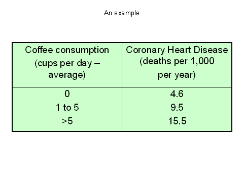
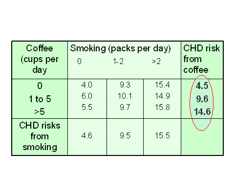
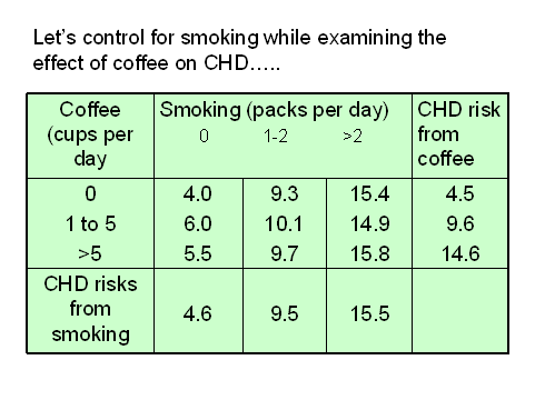
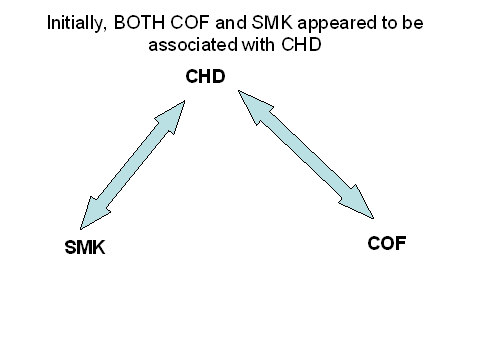
EXAMPLE 1: Is coffee-drinking related to coronary heart disease? .......Several studies have suggested that a link exists between coffee drinking and coronary heart disease. When data are examined, there does appear to be an increased risk of CD among the groups who drink more coffee.
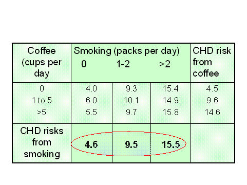
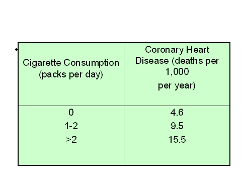
�But when the link between smoking and CHD is plotted,
this variable also seems related to the CHD
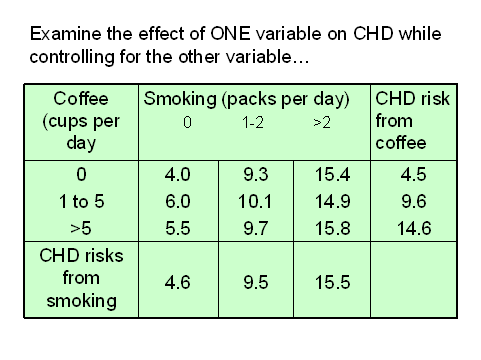
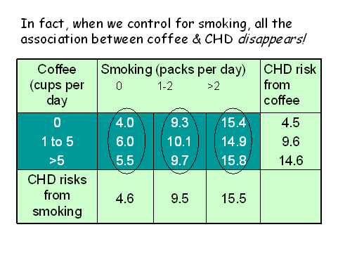
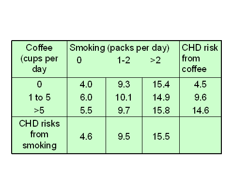
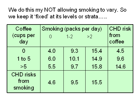
And if we 'control for coffee drinking (by holding it fixed while we
examine the effects of smoking on CHD), we find that the association
between smoking and CHD remains strong!
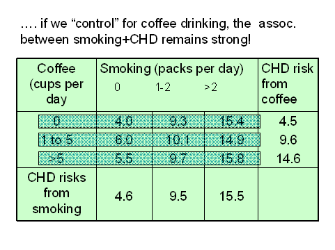
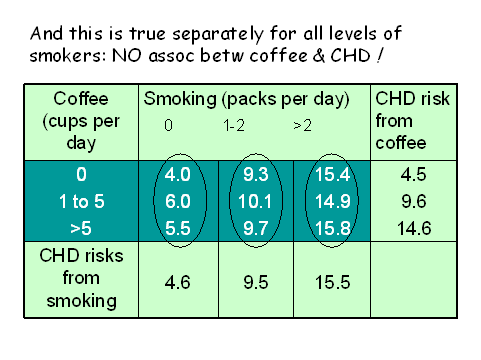
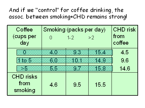
AND this association between smoking and CHD remains
strong at EVERY level of coffee drinking!
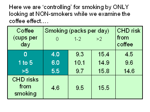
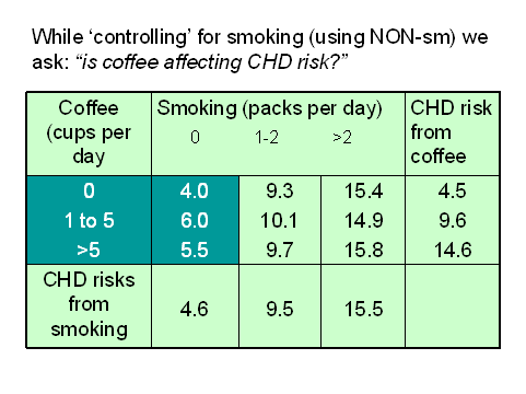
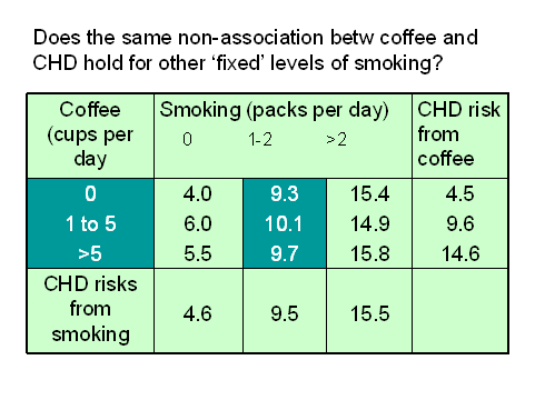
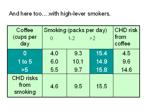
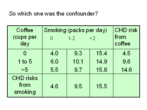
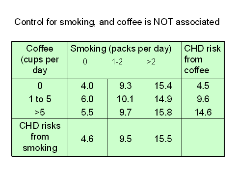
IF we hold SMOKING fixed (CONTROL for SMOKING).....
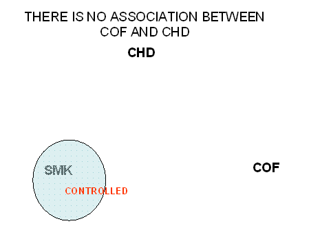
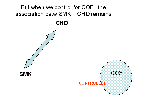
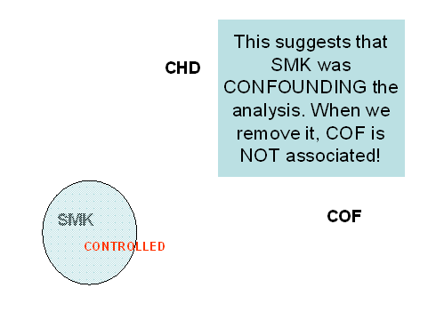
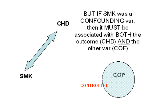
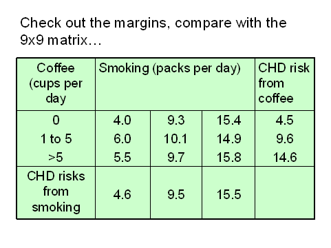
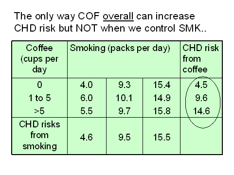
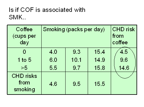
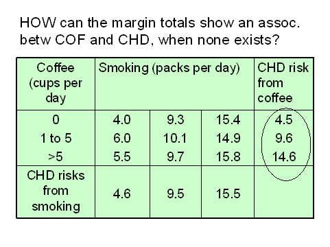
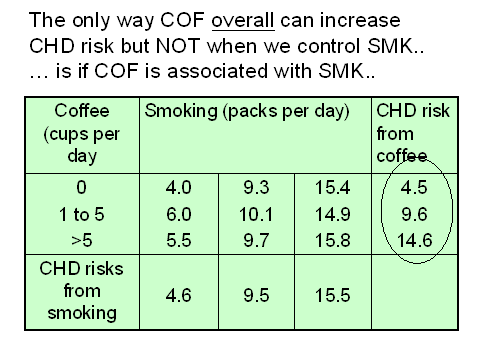
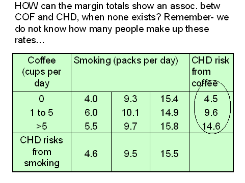
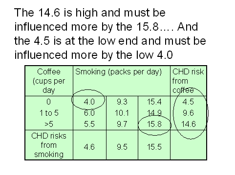
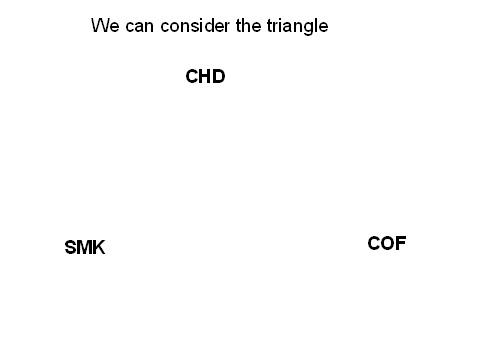
THIS IS IMPORTANT........It means that behind the scenes there are many more people in these cells (hi-smokers + Hi-coffee) and (low-smokers + low-coffee). The conclusion is that Coffee drinking and smoking are associated! In a large population, the tendency (at least at the time this study was done) was that coffee drinking and smoking was a common JOINT practice. Heavy coffee drinkers were more likely to be smokers and vice versa. This means that the third "arrow" can be entered, linking COFFEE and SMOKING........
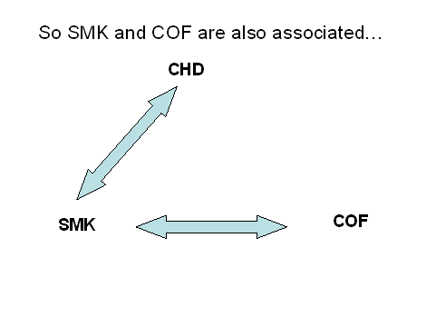
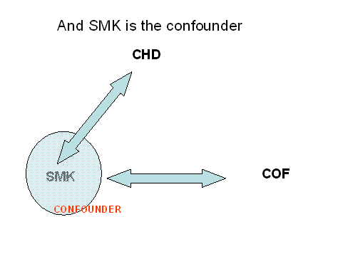
These data mean that coffee is NOT causal for CHD, and that smoking has been acting as a confounding variable, in this case creating a false impression of an association between coffee and CHD. In reality the attention now turns to smoking. It is associated with smoking, and at this stage, seems to be a principle suspect in the search for causes for CHD! Please note: this has now been corrected. There were two errors when this paragraph was first posted. Thanks to Walaa!
__________________________
Example 2: is gender related to genetic damage from occupation?
1. You are presented with data from a study of genetic damage among nearly 8,000 chemical workers. Table 1a shows the average count of genetic damage sites by exposure to chlorinated hydrocarbons; the exposure is categorized as "high", "moderate", and "low".
|
Table
1a.
gender |
Av. No. genetic damage sites |
|
Male Female |
26.8 11.1 |
Table 1b reveals the average count of genetic damage by gender of the workers.
|
Table
1b.
exposure classif |
Av. No. genetic damage sites |
|
high
exp mod exp low exp |
27.3 14.2 9.9 |
Table 1c combines both these tables and allows for a closer inspection of
any confounding variables that may be present.
| Table 1c. Exposure classif. | Gender: male | Gender:female | Both genders combined |
|
high
exp mod exp low exp |
28.3 16.4 10.7 |
26.5 14.0 8.7 |
27.3 14.2 9.9 |
| all exposure groups
|
26.8 | 11.1 |
[A] which of the two variables appears related to the outcome variable before controlling for the other?
Ans: Before controlling, both gender and exposure appear related to gen.damage.
[B] Which of the two variables appears related to the outcome variable after controlling for the other?
Ans: If gender is controlled by stratification (i.e. the relationship betw exp. and gen.damage is examined separately for males and females), a strong, direct, relationship betw exp and gen.damage still exists. Conversely, when exposure is controlled, gender appears to play little or no effect on gen.damage.
[C] Which variable is a confounder? Why?
Ans: Gender cannot be a confounder in this model because it does not appear to be related to the outcome. Exposure may be a confounder because it is related to the outcome, but we would need to show that it is also related to the other input variable, (gender). The table suggests that it is. Look at the overall rates for gen.damage by gender (all exposure levels combined)... 26.8 (M) and 11.1 (F) they do not appear to be representative of all the values in the respective columns above them; the 26.8 seems to be influenced more by the 28.3 than by the 10.7, meaning that there are more males in the high exp. group, and fewer males in the low exp. group. Similarly, there appears to be fewer females in the high exp. group and more in the low exp. group. That is the relationship we are looking for, and this completes the model by which we can state that exposure level was confounding the apparent relationship between gender and genetic damage.
Example 3. Is income related to decision to get a 'flu shot? This study attempts to ascertain whether income level is related to having had been immunized against influenza. In table 2a, the relationship for the whole respondent group (n=500) is shown. In table 2b and 2c, that group is broken down into two age categories: "young" (less than 20 y) and "older" (20y or more).
Table 2a: All respondents
Table 2b: Younger (less than 35y) respondents
Table 2c: Older (35y or more) respondents
|
Table 2a. all respondents |
flu shot | no flu shot | all |
| high income low income |
180 120 |
120 80 |
300 200 |
| all | 300 | 200 | 500 |
| Table 2b. young (<35y) respondents | flu shot | no flu shot | all |
| high income low income |
35 40 |
5 70 |
40 110 |
| all | 75 | 75 | 150 |
| Table 2c. older resp. (35y or more) | flu shot | no flu shot | all |
| high income low income |
160 65 |
100 25 |
260 90 |
| all | 225 | 125 | 350 |
[A] Which variable appears to be the confounder in the above tables? Describe the confounding effect. Ans: Clearly, age group is the confounder because when controlled, the effect of income (INC) upon decision to take a flue shot (FS) has changed. What is missing here is a table showing the relationship betw age and FS and also age and INC.
[B] summarize the effect of not stratifying. Ans: This is an example of a confounder masking the relationship between another variable and the outcome. Uncontrolled for age, the influence of INC on FS is zero. When controlling for age, however, we find that INC does influence FS: for the younger age group, there is a direct and strong influence of INC on FS in that high INC people are more than 12 times as likely to have had a FS than the low INC group. On the other hand, among older respondents, we find that low INC respondents are more likely to have chosen a FS than the high INC. (OR=1.67). If we had not controlled for age, this would have gone unnoticed.
Example 4: Prevalence of antibodies to leptospirosis:
Comparison between urban and rural residents
Table A: Combined genders. From Table A, would you consider that a relationship exists between location and the probability of having been exposed to leptospirosis?
| Antibodies | rural | urban | total |
| yes | 60 (30%) | 60 (30%) | 120 (30%) |
| no | 140 (70%) | 140 (70%) | 280 (70%) |
| total | 200 (100%) | 200 (100%) | 400 (100%) |
Table B: Male only: Do Tables B and C influence your decision?
| Antibodies | rural | urban | total |
|
yes |
36 (72%) | 50 (50%) | 86 (57%) |
| no | 14 (28%) | 50 (50%) | 64 (43%) |
| total | 50 (100%) | 100 (100%) | 150 (100%) |
Table C: Female only
| Antibodies | rural | urban | total |
| yes | 24 (16%) | 10 (10%) | 34 (14%) |
| no | 126 (84%) | 90 (90%) | 216 (86%) |
| total | 150 (100%) | 200 (100%) | 250 (100%) |
4.1 Which variable is the outcome (dependent) variable? LEPTOSPIRAL ANTIBODIES (please note this was previously and erroneously shown as "Gender")
4.2 What are the input (independent) variables? GENDER, LOCATION
4.3 On the basis of these data, would you consider that one variable is confounding another association? YES
4.4 If so, which one is the confounder? GENDER
4.5 Bearing in mind a confounder must be related to the
other input variable as well as the outcome. What is the evidence for this? As Gender seems to affect the association between Location and Antibody measurement, it is by definition a confounding variable. Therefore gender must be related to antibody measurement AND to location. The most likely explanation is the exposure in the fields and ditches by the male farm workers, whereas female jobs did not entail such exposure (to rat urine, etc).
4.6 LOCATION IS RELATED to the outcome (if the GENDER is controlled). If Gender is UNcontrolled, then LOCATION appears to be UNrelated.

