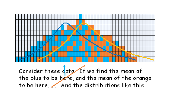
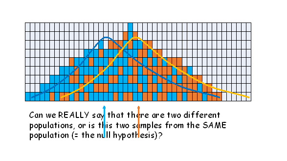
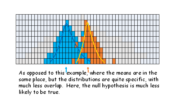
When sampling shows a difference between the means of two groups, the null hypothesis always suggests that no real difference exists between the two groups, and such a difference between the means could have arisen by sampling alone - or two samples taken from the SAME population. The first example shows a wide variance (larger denominator giving a small calc t) and the second a narrow variance (smaller denominator, giving a larger calc t. The essential lesson here is that the denominator is extremely important in generating the t value, and rejecting the null hypothesis.
PART 1:
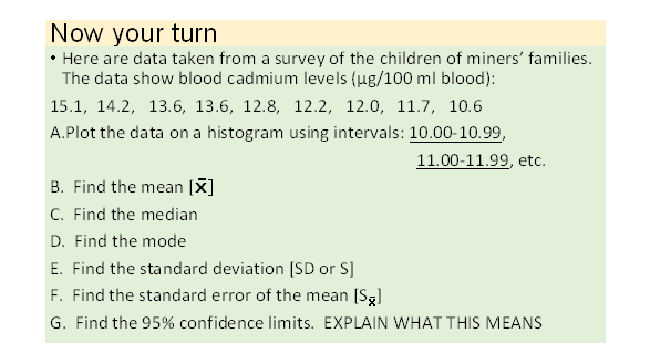
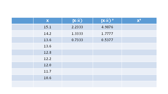
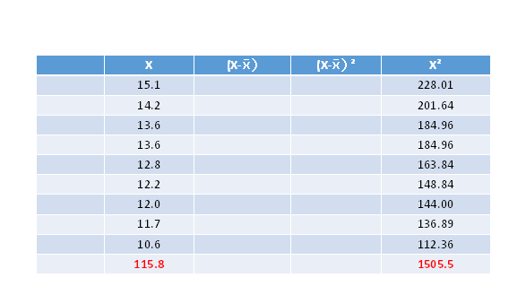
You can certainly complete column 3 to obtain the sum of the squares deviations of each observation from the mean, BUT, it's usually faster and simpler to use the sums of x and x˛
If you did not complete these calculations in class, try it now as a practice before the next test. Make sure you arrive at the correct answers by yourself:
Mean: 12.8667
Median: 12.80
Mode: if you construct the histogram as instructed, the mode occurs in the interval 12.00-12.99
Std Deviation: 1.3937
Std error of the mean: 0.4646
95% conf. Limits: 11.79 to 13.94
Explanation: I do not know the population mean, but from the sample, I am 95% certain that the population mean lies within these limits. This implies that there is a 5% chance the population mean is outside the limits, 2.5% chance that it is less than 11.79, and 2.5% chance it exceeds 13.94.
PART 2
NOW assume that the above was preparing for a comparison of the blood of these children (from families where a parent worked with cadmium) and the blood of children who had no parent working with cadmium. Here are the parameters from BOTH groups"
|
Cadmium workers' children: blood Cadmium level (microgm/100ml blood |
NON- Cadmium workers' children: blood Cadmium level (microgm/100ml blood |
|
| MEAN | 12.8667 | 7.1021 |
| STD DEV | 1.3937 | 1.3122 |
| N | 9 | 9 |
Set up your null hypothesis: "That no real difference exists between the two groups in terms of the blood-cadmium levels; any observed difference is due to chance or random variation"
Now proceed to test the difference between these two means using the t-test for unpaired data that we went through in detail in week 4.
You should be able to derive the following:
The Cadmium workers' children had an average 5.7646 mic.gm/100ml blood MORE than the comparison group children. t(calc): 9.035, 16 df, P<0.001
Interpretation: This difference is unlikely (probability less than 1 in 1000) to have occurred by chance alone. We can safety reject the null hypothesis (that stated "no real difference"), and claim statistical significance at the 0.001 level. We can conclude that children in cadmium workers' families appear to have a very high probability of an elevated cadmium level in the blood.
PART 3:
Use the t-table to find the P (probability values) for the following findings:
1. t = 2.65, 40 df
2. t = 1.99, 60 df
3. t = 1.65, 200 df
4. t = 1.98, 180 df
5. t = 3.72, 28 df
6. Std Eror of the mean: 1.24, difference between means: 2.48, N1= 22, N2: 20
7. mean(1): 9.2, S(1): 1.81, N(1): 62
mean(2): 7.0 S(2): 1.72, N(2): 61
8. t = 1.96, N=1,200
| Answers will be
posted here in a day or so- Try them yourself first and then check to
see how you did.
: Here are the correct probability levels ("rejection values", or "alpha levels"). Knowledge of this process is vital for the study of statistics of every kind. Also note that we are restricted by the t-table being used. The one I am using has alpha levels at 0.05, 0.02, 0.01, 0.005, 0.002, 0.001, so I am responding accordingly. If your table has different alpha (rejection) levels, report the MOST EXTREME (smallest) probability corresponding to the largest critical t value that you were able to meet or exceed. 1. P<0.02 (statistically significant) 2. P>0.05 (not stat. significant) 3. P>0.05 (n.s.) 4. P<0.05 (s.s.) 5. P<0.001 (s.s.) 6. P>0.05 (n.s.) 7. t=6.911, 121 df, P<0.001 (s.s.) 8. P=0.05 (s.s.)
|